 Wed Apr 23 13:05:05 2008, Christian Irmler, SPS Testbeam June08, source, hybrid 01, time correlation between TDC and sensor measurement -> 3.1 ns RMS Wed Apr 23 13:05:05 2008, Christian Irmler, SPS Testbeam June08, source, hybrid 01, time correlation between TDC and sensor measurement -> 3.1 ns RMS 
|
| |
|
Sun Jul 4 05:48:36 2010, Christian Irmler, BELLE Upgrade, source, Origami 6 - module 1, run002: first analysis results 7x
|
Run name: run002
Run type: 0 (Hardware (Normal Run))
Comments:
After ~40min warmup
HV=80
90Sr 1mCi source - moved compared to run001
multi6
Max. Events=100000 Trg delay=25
Origami 6 module #1
w/o cooling
sensor: B2HPK_10938-9239_8
n-side: all 4 APVs read out
p-side: APV #0 to #3 read out, analog output of #4 and #5 were not connected to FADC board
|
|
Wed May 7 15:24:49 2008, Christian Irmler, SPS Testbeam June08, module, module 10/02, properties (noise, intcal), APVs bonded to the sensor 12x
|
| Module tested with 1 and 2 rows bonded to the sensor, respectively.
HV = 100 V
Ibias (100V) = 19.1 nA
Ibias (200V) = 23.7 nA |
|
Wed May 7 15:26:24 2008, Christian Irmler, SPS Testbeam June08, module, module 20/09, properties (noise, intcal), APVs bonded to the sensor 12x
|
| Module tested with 1 and 2 rows bonded to the sensor, respectively.
HV = 100 V
Ibias (100 V) = 25.1 nA
Ibias (200 V) = 31.4 nA |
|
Wed May 7 15:40:07 2008, Christian Irmler, SPS Testbeam June08, module, module 07/07, properties (noise, intcal), APVs bonded to the sensor 12x
|
| Module tested with 1 and 2 rows bonded to the sensor, respectively.
HV = 100 V
Ibias (100 V) = 20.2 nA
Ibias (200 V) = 21.9 nA |
|
Wed May 7 16:12:58 2008, Christian Irmler, SPS Testbeam June08, module, module 12/08, properties (noise, intcal), APVs bonded to the sensor 12x
|
| Module tested with 1 and 2 rows bonded to the sensor, respectively.
HV = 100 V
Ibias (100 V) = 22.2 nA
Ibias (200 V) = 26.5 nA |
|
Wed May 7 19:05:08 2008, Christian Irmler, SPS Testbeam June08, module, module 04/04, properties (noise, intcal), APVs bonded to the sensor 12x
|
| Module tested with 1 and 2 rows bonded to the sensor, respectively.
HV = 100 V
Ibias (100 V) = 27.8 nA
Ibias (200 V) = 32.7 nA |
|
Fri May 9 09:56:15 2008, Christian Irmler, SPS Testbeam June08, module, module 06/03, properties (noise, intcal), APVs bonded to the sensor 12x
|
| Module tested with 1 and 2 rows bonded to the sensor, respectively.
HV = 100 V
Ibias (100 V) = 26.5 nA
Ibias (200 V) = 37.8 nA |
|
Fri May 9 10:00:34 2008, Christian Irmler, SPS Testbeam June08, module, module 03/10, properties (noise, intcal), APVs bonded to the sensor 12x
|
| Module tested with 1 and 2 rows bonded to the sensor, respectively.
HV = 100 V
Ibias (100 V) = 18.9 nA
Ibias (200 V) = 25.5 nA |
|
Fri May 9 10:04:26 2008, Christian Irmler, SPS Testbeam June08, module, module 05/05, properties (noise, intcal), APVs bonded to the sensor 12x
|
| Module tested with 1 and 2 rows bonded to the sensor, respectively.
HV = 100 V
Ibias (100 V) = 18.0 nA
Ibias (200 V) = 23.6 nA |
|
Wed Apr 30 16:52:17 2008, Markus Friedl, BELLE Upgrade, module, micron, micron sensor glued to frame
|
soeben haben wir den micron-DSSD (double metal layer) in den 2-teiligen rahmen geklebt und auf beiden seiten
temporäre kapton-stückerln aufgeklebt, über die bias appliziert werden kann. nach trocknung und bonden der
bias-verbindungen (montag, 5.5.2008) wird dieser für sensor-tests zur verfügung stehen. |
|
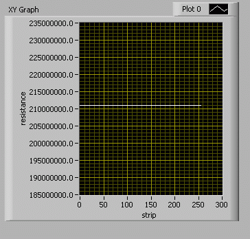
Wed Oct 7 14:23:35 2009, Dieter Uhl, BELLE Upgrade, hybrid, #4, hybrid-pitchadapter
|
opens at upper coat
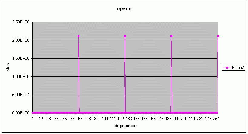
shorts at upper coat
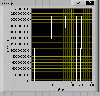
opens at lower coat
shorts at lower coat
|
|
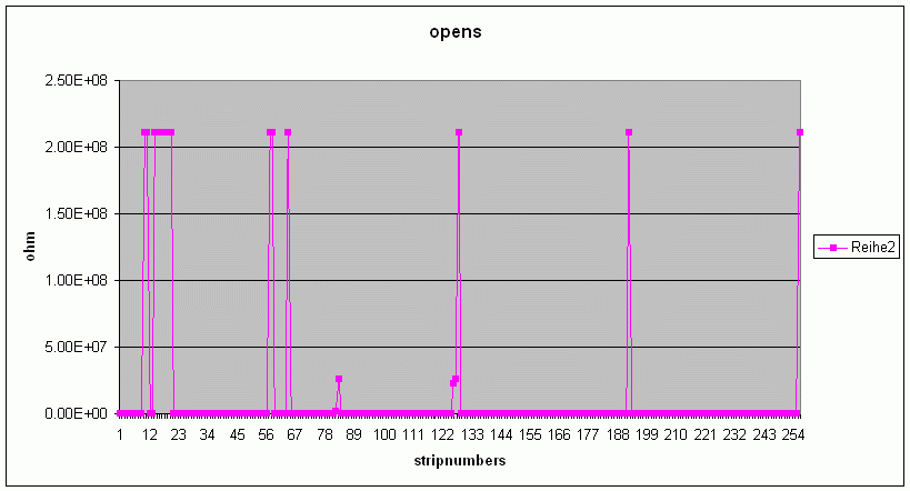
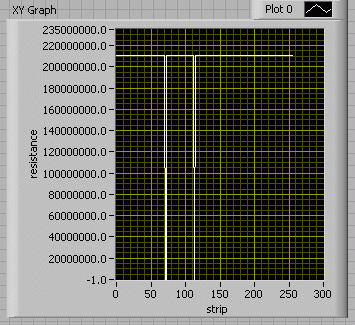
Wed Oct 7 14:24:06 2009, Dieter Uhl, BELLE Upgrade, hybrid, #5, hybrid-pitchadapter
|
shorts at upper coat
opens at upper coat
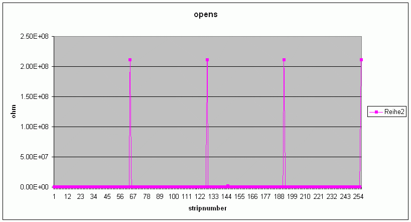
shorts at lower coat
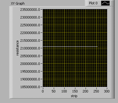
opens at lower coat

|
|
Wed Apr 23 13:37:18 2008, Markus Friedl, SPS Testbeam June08, source, hybrid 01, analysis results of source test
|
Ignore the "KEK November 2007" title - that's a legacy and is already changed :-)

As of now, there is no distinction in 16 separate zones. However, the gaps between the the zones are clearly visible in the Hit Profile, as the edge strips on both sides have a larger sensitive area and thus collect more hits than other strips; hence the spikes in the (otherwise pretty gaussian) beam profile. There is a single strip with no entries in the center - that's the one that suffered from the bias bond repair action.
SNR=21 (peak mode) is pretty healthy and fits to similar detectors operated with APV25.
All data was taken in multi-peak mode with subsequent hit fitting to obtain amplitude and timing (see separate posting for timing precision).

The verbose output of the analysis is pasted below.


Analysis of vie_run001

Peak Mode, 3 x 200 initevents (first 10 skipped) + 99400 events
Number hybrids:  1	number zones:  2	 number sensors:  1
Using calibration file vie_cal001
No pedestal correction file
Seed/Neighbor/Cluster/Noisy Strips Cuts [RMS noise]: 5.0/3.0/5.0
Min. hitlength:   3


Comments:
SILC module 01
HV=100V, 40MHz, Tp=50ns, 30ns
Sr90 1mCi ,  black cloth cover


Analysis date: 23.04.2008 13:25:09


Analysis settings:
 runname: vie_run001_cluster
 clock: 40.00 MHz
 datafilepath: data/
 outputpath: output/
 subevents:  6
 fitmode: 2 (cal. fit)
 options: h


Results:

ModuleName           ZoneType    Ch    OKCh     OK%   Entries    MClW    MPSignal   Noise   MPSNR   HpSE  Occup
p_side JP single sensor 256 256 100.0 90385 2.53 21546.1 729.4 20.68 0.53 1.81 |
|
Tue May 20 14:27:50 2008, Markus Friedl, BELLE Upgrade, source, micron, analysis results of source test 9x
|
*** NOTE: AFTER THIS MEASUREMENT WE REALIZED THAT BIASING WAS NOT DONE PROPERLY
          HENCE THE RESULTS BELOW ARE NOT RELIABLE
          (in fact it is surprising that they are not worse) ***


Please find the results of the lab source test on the new Micron module here.
It is read out with 3 + 3 APV chips on either side.

Results table of the source measurement:
                      p-side     n-side
 Cluster signal [e]    18361      19434
 Strip noise [e]        1142       1193
 Avg cluster width      1.91       1.30
 Single strip SNR       16.1       16.3
 Cluster SNR            11.6       14.3
 Strip pitch [um]       50.0      153.5

Apparently, the double metal capacitance is not so bad as expected, even though the Micron sensor does not use
the hourglass crossing scheme. Presumably the dielectric between metal 1 and 2 is rather thick (several um).
Strip noise is roughly the same on both p and n side, so the difference in Cluster SNR (*) only stems from the
unequal cluster width (which is a result of the different pitches).

Peak time precision vs SNR (last plot below) is worse compared to the values obtained with various HPK sensors
in the November 2007 beam test at KEK. However, this is a comparison of source and beam and thus might not be
significant. Let's see what we will get in the SPS beam test next week.

(*) Cluster SNR := sum(signal) / (strip_noise * sqrt(cluster_width) ) |
 Fri May 29 11:47:56 2015, Hao Yin, Belle II, system, PS Filter, Testing PS LV filter and quantifying the required min noise lvl
|
Data of this entry is recorded in the folder: LV315kHz_Injections
Injecting noise to LV with a freq. of 314 kHz to emulate Caen PS with KenWood PS.
Run Name 315kHzKenWood_: (injecting cmc noise into p-side lv) (attachment 1)
000 ... baseline noise
001 ... 4mA
002 ... 1mA
003 ... 1mA wo Amplifier
004 ... 4mA wo Amplifier
005 ... 0.5mA wo Amplifier
006 ... 2mA wo Amplifier
007 ... 0.2mA wo Amplifier
Run Name 315kHzKenWood_Filter_BW_: (injecting cmc noise into p-side lv with filters (inductance with 470 mH x 6 ) conn. at bw) (attachment 1) (wo Amplifier)
000 ... baseline noise
001 ... 0.2mA
002 ... 0.4mA
003 ... 0.5mA
004 ... 1mA
005 ... 2mA
006 ... 4mA
Run Name 315kHzKenWood_Filer_BW_HVRET-GND:
000 ... baseline noise
001 ... 0.2mA
002 ... 0.4mA
|
|
Thu Jun 5 10:34:29 2014, Benedikt Würkner, Belle II, source, Silc Module, Silc Angle Measurement 7°
|
Measured the Silc 03/10 Module using the Sr90 Source to have a comparison for the Eta-Distribution at different angles.
Data can be found on heros in: /home/medialib/LAB_Silc_Angle.
Plots made with TuxOA for all different regions can be found in /home/users/bwuerkner/plots/.
|
|
Thu Jun 5 10:34:06 2014, Benedikt Würkner, Belle II, source, Silc Module, Silc Angle Measurement 4°
|
Measured the Silc 03/10 Module using the Sr90 Source to have a comparison for the Eta-Distribution at different angles.
Data can be found on heros in: /home/medialib/LAB_Silc_Angle.
Plots made with TuxOA for all different regions can be found in /home/users/bwuerkner/plots/.
|
|
Thu Jun 5 10:33:46 2014, Benedikt Würkner, Belle II, source, Silc Module, Silc Angle Measurement 1°
|
Measured the Silc 03/10 Module using the Sr90 Source to have a comparison for the Eta-Distribution at different angles.
Data can be found on heros in: /home/medialib/LAB_Silc_Angle.
Plots made with TuxOA for all different regions can be found in /home/users/bwuerkner/plots/.
|
|
Thu Jun 5 10:34:45 2014, Benedikt Würkner, Belle II, source, Silc Module, Silc Angle Measurement 10°
|
Measured the Silc 03/10 Module using the Sr90 Source to have a comparison for the Eta-Distribution at different angles.
Data can be found on heros in: /home/medialib/LAB_Silc_Angle.
Plots made with TuxOA for all different regions can be found in /home/users/bwuerkner/plots/.
|
|